The Heisenberg Uncertainty Principle, although well known in the pop science genre, it is not understood mathematically by most.

This is highly due to the fact that the Quantum realm is thought of as the Pandora's box in physics. In this article we'll explain the uncertainty principle using just two postulates of Quantum Mechanics. The only prerequisites would be to be familiar with matrices and complex number algebra, as the rest is derived from there onward. Eigen-stuff and the Cauchy-Schwarz inequality will be used to introduce the topic. Disclaimer: This is only intended to be an introduction to Quantum Mechanics, and a conversation starter, as the topic is much more math heavy when studied in detail.

Quantum Mech 101

When we use the word "Postulate", we mean that it is a principle from the which the rest of the theory can be constructed. So here are the postulates for Quantum Mechanics that we will consider.

The State Vector

The state vector is an object represented as

$$| \psi \rangle$$

This is known as a "Ket" or column vector. We can extract maximal information (i.e. as much as we can. This is not necessarily everything) about the system by applying operations to it, thus there is by nature an unpredictability about the future of the system. This is in stark contrast (or maybe not) to classical physics, where knowing the state of something corresponds to knowing everything that can be known about it. The obvious question to ask is, "whether the unpredictability is due to an incompleteness in the a quantum state or is it due hidden variables that are inaccessible to us?". There are various opinions about this matter, this is still an open issue. However, for now we'll act as if there is an inherent unpredictability (despite newer theories having deterministic features) . This approach is called the "Copenhagen interpretation". Another interesting thing that we could do is express the state vector as a superposition of other states:

$$| \psi\rangle = \alpha |\psi_1 \rangle + \beta |\psi_2 \rangle$$

Provided the complex numbers $\alpha$ and $\beta$, satisfy the condition $$\alpha {\alpha}^{*} + \beta {\beta}^{*} = 1$$

They are said to be normalized, we impose this condition because the complex conjugation represents the probability of something occurring and we want to ensure that all the probabilities add up to 1. Where the $*$ symbol represents complex conjugation. Similarly we can introduce a row vector called the "Bra", but however, since the elements are complex numbers we need to conjugate them as well

$$ \langle\psi | = |\psi\rangle^{\dagger} = {(|\psi\rangle^{*})}^{T} = \begin{pmatrix}\psi^{*}_1  \ \psi^{*}_2 \end{pmatrix} $$

Where $T$ represents the transposition of a matrix and the $\dagger$ (dagger) represents complex conjugation followed by transpose. We can write it as,

$$\langle \psi | \psi \rangle = \begin{pmatrix} \psi^{*}_1 \ \psi^{*}_2 \end{pmatrix}\begin{pmatrix} \psi_1 \\ \psi_2 \end{pmatrix}$$

$$\langle \psi | \psi \rangle = \psi_1 \psi^{*}_1 +  \psi_2\psi^{*}_2$$

This can still have negative numbers, so we take absolute value of it. However, this still doesn't represent probabilities since . Thus, we square it. This is analogous to finding the square of the length of the vector representing $\psi$,

$$|\langle \psi |\psi\rangle | ^{2} = 1$$

This is called the "Born rule", as it was first suggested by Max Born.

Observables

We can apply operations to the state vector to find out what happens to measurable quantities such as momentum and position. The operations are termed as operators and are represented using matrices

$$\hat{O} = \begin{pmatrix} O_{11} & O_{12}\\ O_{21} & O_{22} \end{pmatrix}$$

These operators are termed linear that is they follow the properties:

$$\hat{O} (\alpha |\psi\rangle) = \alpha \hat{O} |\psi\rangle$$

$\forall \ \alpha \in \mathbb{C}$. $\forall$ indicates "for all" and $\in$ as  Read in continuity, they mean "for all values in a set $\mathbb{C}$, the set of all complex numbers".

$$(\hat{O}_1 + \hat{O}_2)|\psi\rangle = \hat{O}_1|\psi\rangle+ \hat{O}_2 |\psi\rangle \\ \hat{O} (\alpha |\psi\rangle) = \alpha \hat{O} |\psi\rangle$$

For example the momentum operator is given by the equation

$$\hat{P} = -i \hbar \frac{\partial}{\partial x}$$

where $i$ is the imaginary number, and $\hbar = \frac{h}{2 \pi}$ a physical constant ($h$ is called Planck's constant) with the dimensions . So if we look at how it operates it is easy to see that

$$\hat{P}|\psi\rangle = -i \hbar \frac{\partial | \psi \rangle}{\partial x}$$

Math interlude: Matrices

Matrix Multiplication

When we multiply two number A and B for instance, we have this property

$$AB = BA$$

this is called as commutativity. However, when deal with operators we're dealing with matrices, so in general

$$\hat{A}\hat{B} \neq \hat{B}\hat{A}$$

But in a few cases two operators can commute, thus we use a measure called the "Commutator" to quantify if or not two operators commute

$$[\hat{A}, \hat{B}] = \hat{A}\hat{B} - \hat{B}\hat{A}$$

Thus, if the commutator is 0 then the operators commute, if not then they don't commute. satisfied. Moreover we can represent the multiplication of a Bra and a Ket as,

$$\langle X|Y \rangle = \langle X | \  |Y\rangle = \begin{pmatrix} x_1 \ x_2 \end{pmatrix} \begin{pmatrix} y_1 \\ y_2 \end{pmatrix}$$

and it is quite easy to see that

$$\langle X | X \rangle = |X|^2$$

Eigen-stuff

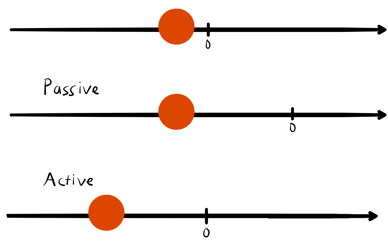
Since operators are basically matrices, we can also have the "transformation" picture in mind. That is, when I multiply a vector or in this case the state vector with a matrix I make a change to it. This can be visualized as a passive transformation i.e. change of coordinates or an active transformation i.e. the state vector's position is transformed.

Most of the time the , but there are a few vectors such that their direction remains unchanged, they are called Eigenvectors. Their direction isn't changed however there is no constraint on how the length is changed, so sometimes their length is scaled up or down by multiplying it with a real number called an Eigenvalue. For a more intuitive explanation, check out this video by 3Blue1Brown

That is in summary, the effect the operator has on that particular vector is equal to multiplying it by a real number.

$$\hat{O} |\lambda\rangle = \lambda |\lambda\rangle$$

What does this mean for Quantum Mechanics? Each Eigenvalue represents something that can be measured by applying that operator. More importantly, this will always be a real number as we can only measure real numbers. For more deep dive into Eigen-stuff head to this article on Eigendecomposition.

Math interlude: Statistics

In Quantum Mechanics we can only make probabilistic predictions so we will deal with probability quite much. Through that we can define the average of a possible values $\lambda_i$ measured by an operator $\hat{A}$

$$\langle \hat{A} \rangle = \sum_{i} \lambda_i P(\lambda_i)$$

Where $P(\lambda_i)$ represents the probability of that particular to be measured. We can rewrite this in terms of a state vector $| \psi \rangle$

$$\langle\psi | \hat{A} |\psi \rangle= \sum_{i}^{} \lambda_i P(\lambda_i)$$

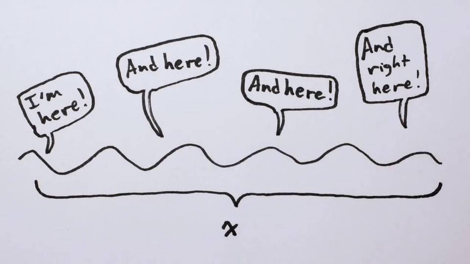
What we mean by uncertainty is simply how much a particular value or a variable in general deviates from the mean, this is captured using the statistical quantity "standard deviation". To define it first we define a new operator such that

$$\bar{A} = \hat{A} - \langle \hat{A}\rangle I$$

whose Eigenvalues are defined by

$$\bar{\alpha} = \alpha - \langle \hat{A} \rangle$$

We can now define the uncertainty or standard deviation of $\hat{A}$ which we call $\sigma^{2}_{A}$ as

$$\sigma^{2}{A} = \sum_{i}^{} \bar{\alpha}^{2} P(\alpha)$$

or as,

$$\sigma^{2}{A} = \sum{i} (\alpha_i - \langle \hat{A}^{2} \rangle)^{2}P(\alpha_i)$$

Now if we assume $\langle \hat{A} \rangle = 0$, that is to say that the distribution $\langle\hat{A} \rangle$ is symmetric, then

$$\sigma_{A}^{2} = \sum_{i}^{} \alpha_{i}^{2} P(\alpha_{i})$$

Which can be written as,

$$\sigma^{2}_{A} = \langle \psi | A^{2} |\psi \rangle = \langle A^2 \rangle$$

Math interlude: Cauchy-Shwarz inequality

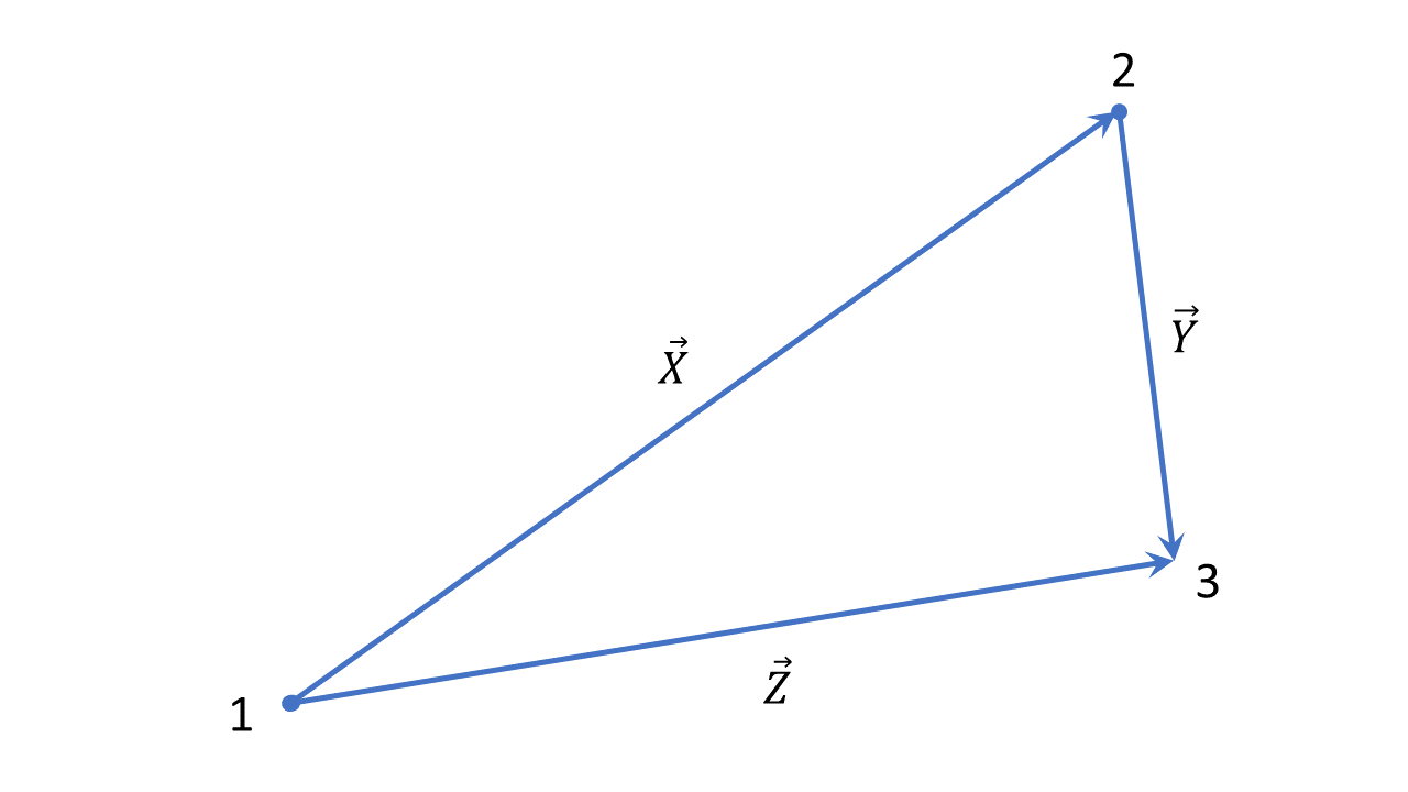
For all triangles as depicted above,

$$|X| + |Y| \geq |Z|$$

Where |X| is the length of the vector $\vec{X}$. We can also write the last equation as:

$$|\vec{X}| + |\vec{Y}| \geq |\vec{X} + \vec{Y}|$$

Squaring this equation it becomes,

$$|\vec{X}|^2 + |\vec{Y}|^2 + 2|\vec{X}||\vec{Y}| \geq |\vec{X} + \vec{Y}|^2$$

Expanding the right side we get,

$$|\vec{X}|^2 + |\vec{Y}|^2 + 2|\vec{X}||\vec{Y}| \geq |\vec{X}|^2 + |\vec{Y}|^2 + 2(\vec{X}.\vec{Y})$$

Cancelling the terms we find,

$$|\vec{X}||\vec{Y}| \geq \vec{X}.\vec{Y}$$

This is called the Cauchy-Schwarz inequality. Writing this using the state vectors, $$|X| = \sqrt{\langle X| X \rangle}$$

$$|Y| = \sqrt{\langle Y| Y \rangle}$$

$$|X + Y| = \sqrt{(\langle X | + \langle Y |)(|X\rangle + |Y\rangle)}$$

we have by substituting into the inequality,

$$\sqrt{\langle X| X \rangle} + \sqrt{\langle Y | Y \rangle} \geq \sqrt{\langle X|Y \rangle + \langle Y|X \rangle}$$

squaring it and simplifying we find

$$2|X||Y| \geq |\langle X|Y \rangle + \langle Y|X \rangle |$$

This is the Cauchy-Schwarz inequality written in terms of state vectors.

The Uncertainity Principle

Suppose we have a ket $| \psi \rangle$ and two operators $\hat{A}$ and $\hat{B}$, we define their standard distribution as

$$\sigma^{2}_{A} = \langle f | f \rangle$$

$$\sigma^{2}_{B} = \langle g | g \rangle$$

Where,

$$| f \rangle = (\hat{A} - \langle A \rangle)| \psi \rangle$$

$$| g \rangle = (\hat{B} - \langle A \rangle)| \psi \rangle $$

We use the Cauchy-Shwarz inequality,

$$\sigma^{2}_{A} \sigma^{2}_{B} = \langle f  | f \rangle \langle g | g \rangle \geq  {|\langle f|g \rangle|}^{2}$$

And for any complex number $z$,

$${|z|}^{2} = {[Re(z)]}^{2} + {[Im(z)]}^{2} \geq {[Im(z)]}^{2}$$

We then set, $z = \langle f | g \rangle$

$$\sigma^{2}_{A} \sigma^{2}_{B} = {\left(\frac{1}{2i} [ \langle f | g \rangle - \langle g | f \rangle]\right)}^{2}$$

But

$$\langle f | g \rangle = \langle \psi | ( \hat{A} - \langle A \rangle ) (\hat{B} - \langle B \rangle) | \psi \rangle$$

$$\langle f | g \rangle = \langle \hat{A}\hat{B} \rangle - \langle \hat{B} \rangle \langle \hat{A} \rangle - \langle \hat{A} \rangle \langle \hat{B} \rangle + \langle \hat{A} \rangle \langle \hat{B} \rangle$$

$$\langle f | g \rangle = \langle \hat{A}\hat{B} \rangle - \langle \hat{B} \rangle \langle \hat{A} \rangle - \langle \hat{A} \rangle \langle \hat{B} \rangle + \langle \hat{A} \rangle \langle \hat{B} \rangle$$

$$\langle f | g \rangle = \langle \hat{A}\hat{B} \rangle - \langle \hat{A} \rangle \langle \hat{B} \rangle$$

Therefore,

$$\langle g | f \rangle = \langle \hat{B}\hat{A} \rangle - \langle \hat{A} \rangle \langle \hat{B} \rangle$$

We can then say that,

$$\langle f | g \rangle - \langle g | f \rangle = \langle \hat{A}\hat{B}\rangle -  \langle \hat{B}\hat{A}\rangle= \langle \psi | \hat{A}\hat{B} - \hat{B}\hat{A} | \psi \rangle$$

Which is the same as,

$$\langle f | g \rangle - \langle g | f \rangle = \langle [\hat{A},\hat{B}] \rangle$$

Putting this all together we get,

$$\sigma^{2}_{A} \sigma^{2}_{B} \geq {\left(\frac{1}{2i}\langle [\hat{A},\hat{B}] \rangle\right)}^{2}$$

This is called the generalized uncertainty principle. This basically states that two variables that do not commute cannot be measured with precision simultaneously.

Talking about position and momentum

We know that observable properties can be represented using operators, here we'll

$$\hat{x} = x$$

$$\hat{P} = -i\hbar \frac{\partial}{\partial x}$$

So we now try to find the commutator of those operators now

$$[\hat{x}, \hat{p}] = \hat{x}\hat{p} - \hat{p}\hat{x}$$

$$[\hat{x}, \hat{p}] = -ix\hbar \frac{\partial}{\partial x} + i\hbar \frac{\partial}{\partial x}$$

Now let's apply this to state vector to obtain the expectation value

$$[\hat{x}, \hat{p}] |\psi\rangle = -ix\hbar \frac{\partial}{\partial x} |\psi\rangle + i\hbar \frac{\partial x|\psi\rangle}{\partial x}$$

$$[\hat{x}, \hat{p}] |\psi\rangle = -ix\hbar \frac{\partial}{\partial x} |\psi\rangle + ix\hbar \frac{\partial |\psi\rangle}{\partial x} + i\hbar$$

$$[\hat{x}, \hat{p}] |\psi\rangle = i\hbar$$

Substituting this into the generalized uncertainty principle,

$$\sigma_{x}\sigma_{p} \geq \frac{1}{2i} i\hbar$$

$$\sigma_{x}\sigma_{p} \geq \frac{\hbar}{2} $$

$$\sigma_{x}\sigma_{p} \geq \frac{h}{4 \pi}$$

Capping it all off

We can visualize all of this in the form of waves. The more precisely we measure its wavelength

the less precisely we measure its frequency.

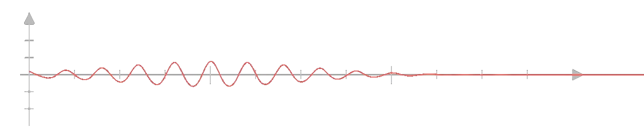
Thus, the state vector can be thought of a wave whose frequency and wavelength somehow correspond to position and momentum or it is simply a wave in a space where the axes are position and momentum. The uncertainty principle thus isn't just a property of quantum Mechanics but is a property of waves in general.

Acknowledgements

We would like to thank Chinmaya Bhargava and Samarth Mishra for picking out errors in the draft.

References

1. Susskind, L. and Friedman, A. Quantum Mechanics: The Theoretical Minimum. Basic Books, 2014
2. Schwichtenberg, Jakob. No-Nonsense Quantum Mechanics: a Student-Friendly Introduction. No-Nonsense Books, 2019
3. Jakob, Demystifying Gauge Symmetry