Disentangling Entanglement

Quantum mechanics is one of the recent topics in modern physics. Since its establishment as a field in physics, it has revolutionized our understanding and interpretation of nature and how the particles behave in scales smaller than an atom. This theory was developed in the early 20th century in order to explain the various quantum scale phenomenon that was observed by various pioneer physicists of the time like JJ Thomson, Albert Einstein, Niels Bohr, Max Planck, etc. Ever since then, physicists have continued to further understand this mysterious realm and the deeper we went the darker our understanding became where the existing laws of physics just didn’t make sense. In this article, we’ll try to make sense of the concepts of “Spin” and “Quantum Entanglement”. The specialty of these concepts is that there no classical analogies for them, and they are only applicable to the quantum mechanical systems.
Math!
Without further ado, let's set up the mathematics behind entanglement first! To start off, let's look at some of the "fancy" math symbols we commonly use:
| Symbol | Meaning |
|---|---|
| $\forall$ | For all |
| $\exists$ | There exists a |
| $\in$ | In |
| $|$ or : | Such that |
| := | Defined as |
| $\rightarrow$ | Maps to |
we will often use them to succinctly and precisely represent the ideas. We will simply review the underlying mathematics and not prove things. However, if you wish to see the proofs, you can consult any of the references.
Vector Spaces
A linear vector space or simply a vector space $\mathbb{V}$ is a set along with the multiplication $(.)$ and addition $(+)$ operations defined over a field $F$ (set of all complex numbers $\mathbb{C}$), such that the following axioms hold:
- Commutativity: $| U \rangle + | V \rangle = | V \rangle + | U \rangle$
- Associativity: $(| U \rangle + | V \rangle) + | W \rangle = | V \rangle + (| U \rangle + | W \rangle)$
- Additive Identity: $\exists \ | 0 \rangle \in \mathbb{V} \ | \ | V \rangle + | 0 \rangle = | 0 \rangle + | V \rangle = | V \rangle$
- Additive Inverse: $\forall \ | V \rangle \ \exists \ | V^{-1} \rangle \ | \ | V \rangle + | V^{-1} \rangle = 0$
- Multiplicative identity: $\exists \ \alpha \in \mathbb{C} \ | \ \alpha . | V \rangle = | V \rangle$
- Distributive properties:
- $(\alpha + \beta) | U \rangle = \alpha | U \rangle + \beta | U \rangle$
- $(\alpha \beta) | V \rangle = \alpha (\beta | V \rangle)$
Here, $\alpha , \beta \in F$ and $| U \rangle,| V \rangle,| W \rangle \in \mathbb{V}$. For more, check out
Dual Space
Every vector space $\mathbb{V}$ has a dual space $\mathbb{V}^{*}$ whose elements map elements of $\mathbb{V}$ to $\mathbb{R}$ i.e.
$$\forall \ |V\rangle \ \exists \ \langle W| \in \ \mathbb{V}^{*}: \langle W|:= |V\rangle \rightarrow F$$
Now, given such a map $\phi\in V^*$ and a vector $|v\rangle$, it is always possible to 'evaluate' the vector via $\phi(|v\rangle)$. This is natural in the sense that no other structure is needed to define this (contrast this with the isomorphism $V\to V^*$ which requires construction of a basis of $V$, which is indeed an extra structure). This evualutaion is defined more formally as a duality.
A duality is a triple $(X,Y,f)$ over the field F consisting of two vector spaces $X$ and $Y$ over $F$ and a bilinear map $f:X\times Y\to K$ such that $\forall X\ni x\ne 0,\ Y\ni y\mapsto f(x,y)\ne 0$ and vice versa. So, the triple $(V,V^*,f)$ is indeed a duality where $f$ is the evaluation map, that is $f(|v\rangle,\langle w|)=\langle w||v\rangle.$
Why is this important? Well because once we say that our vector spaces are indeed Hilbert spaces, one can define $\langle w||v\rangle:=\langle w|v\rangle$ as the natural inner product on the space! This along with completion (to be defined later) would ultimately say that for any $\phi\in V^*$, there exists a unique vector $|v_\phi\rangle$ such that $\phi(x)=\langle v_\phi|x\rangle$ for all $x\in V$. This is the famous Riesz representation theorem. This then automatically gives us a semi-bilinear (linear in first argument, anti-linear in second) map from $V$ to $V^*$. The map is $$\phi:V\to V^*\ \ \text{defined by}\ \ y\to \phi_y=\langle\cdot|y\rangle$$ Riesz gurantees this map is bijective and hence Dirac's famous result that every vector $|v\rangle$ has a dual $\langle v|$.
The Inner Product
Inner product is a generalization of the dot product that we are familiar with. It is defined as follows, the operation $\langle . | . \rangle$
- Skew-symmetry: $\langle V | W \rangle = { \langle W | V \rangle}^{*}$
- Positive semidefiniteness: $\langle V | V \rangle \geq 0$, unless and until $| V \rangle = | 0 \rangle$
- Linearity for the vectors: $\langle U | (\alpha | V \rangle+\beta | W \rangle) = \langle U | \alpha | V \rangle + \langle U | \beta | W \rangle = \alpha \langle U | V \rangle+ \beta \langle V | W \rangle$
Where, $\alpha \in \mathbb{C}$ and $| U \rangle,| V \rangle,| W \rangle \in \mathbb{V}$ and $\langle U| ,\langle V |, \langle W| \in \mathbb{V}^{*}$
Linear Maps
A linear map/transformation is simply transformation $\hat{O}$ that
- Adds inputs or outputs, $\hat{O}(\vec{V} + \vec{W}) = \hat{O}(\vec{V}) + \hat{O}(\vec{W})$
- Scale the inputs or outputs, $\hat{O}(\alpha \vec{V}) = \alpha \hat{O}(\vec{V})$
Here, $\alpha , \beta \in \mathbb{C}$ and $| U \rangle,| V \rangle, | W \rangle \in \mathbb{V}$
Cartesian Product
Here the symbol "$\times$" means "Cartesian Product" i.e. it's action w.r.t two sets is the set of all ordered pairs $(a, b)$ where $a \in \mathbb{A}$ and $b \in \mathbb{B}$
Tensor Product
The tensor product $v \otimes w \ \forall \ v \in \mathbb{V}, w \in \mathbb{W}$ is an element of the set $\mathbb{V}^{*} \times \mathbb{W}^{*}$ i.e. the set of all Bilinear functions on which act on the pair $(h,g) \in \mathbb{V} \times \mathbb{W}$.
Hilbert Spaces
A Hilbert space is a vector space $\mathcal{H}$ that
- has an norm i.e. length defined as $||V|| = \sqrt{\langle V | V\rangle}$
- is complete i.e. all of it's Cauchy sequences converge
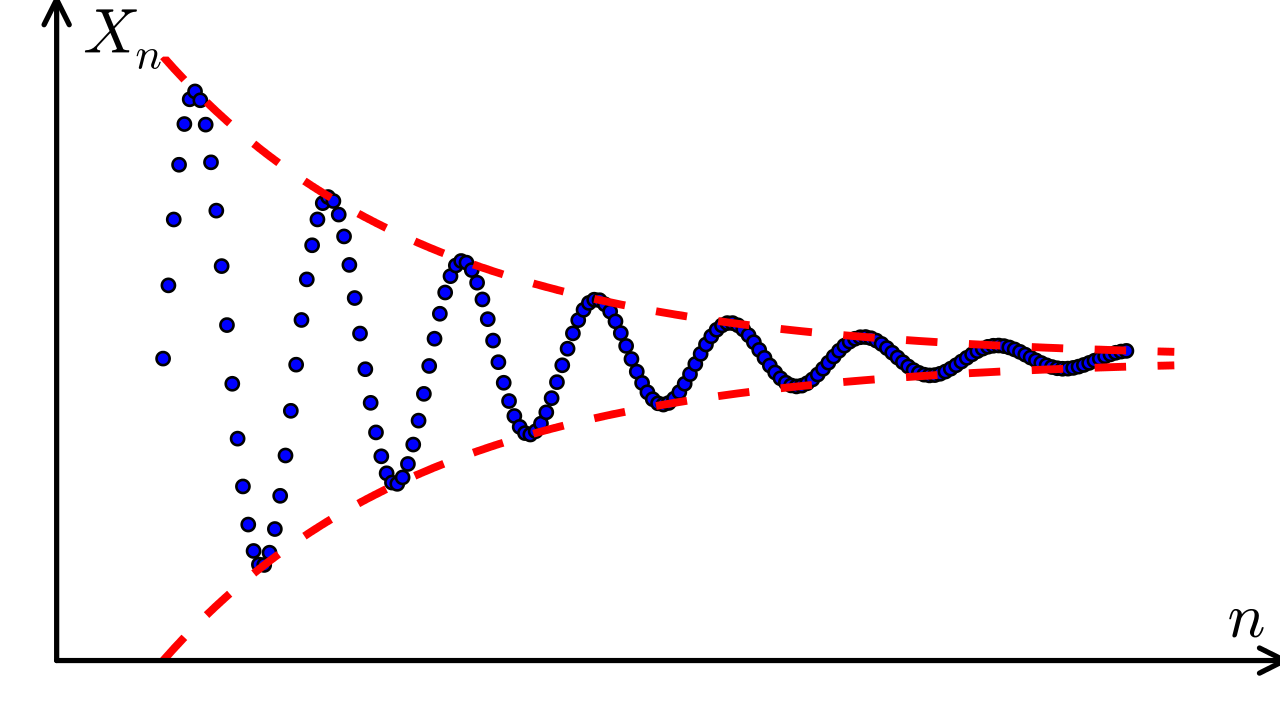
A Cauchy sequence is simply a sequence of numbers whose succeeding term is smaller than the preceding one and when taken to a limit it converges. Let's take a sequence $a_{1},a_{2}... a_{n}$. A function $d(a_{m},a_{n})$ tells us the distance between the terms $a_{m}$ and $a_{n}$, we can call it a Cauchy sequence if
$$\lim_{min(m,n) \rightarrow \infty} d(a_{m},a_{n}) = 0$$
One can visualize this as the plot of a dampened oscillator.
Quantum Mechanics 101
Now that the general math concepts (which we will be heavily relying on in the upcoming sections) have been established, we can now try to dive deeper into the technical aspects of a quantum mechanical system using the aforementioned concepts.
The State Vector
In Quantum Mechanics, we start with an object called the state vector $| \psi \rangle \in \mathcal{H}$
- All the information about the system is contained in it
- The position basis representation of the state vector is called the wavefunction $\psi (\vec{x}, t) = \langle x | \psi \rangle$
Observables
In Quantum Mechanics, observable quantities such as position and momentum are promoted to Linear maps i.e. observables. Acting with an observable on a state vector will allow you to measure the physical quantity that corresponds to the map. These maps are Hermitian/Self-Adjoint i.e.
$$\hat{O} = \hat{O}^{\dagger} = {(\hat{O}^{*})}^{T}$$
Where $*$ refers to complex conjugation and the $T$ to the transpose operation i.e swapping the rows and columns. The observable values of a particular quantity come in are the eigenvalues from the eigenvalue equation (here the operation of the observable simply scales or changes the length of the state vector) of the map acting on a state vector i.e. and such state vectors that obey this equation are called eigenvectors or eigenstates
$$\hat{O} | \psi \rangle = \lambda | \psi \rangle$$
Few Corollaries:
The eigenvalues are always real numbers
The eigenstates form an orthonormal (perpendicular and normalized i.e. of length 1) basis set
$$ \langle \lambda_{i} | \lambda_{j} \rangle = \delta_{ij} \begin{cases} 1, & \text{if } i=j \ 0, & \text{if } i \neq j \end{cases} $$
However, the catch is that we can't definitively say that we will measure a particular eigenvalue since quantum mechanics (at least as we understand it) is probabilistic. So we rely on Born's rule to compute probabilities for a given eigenstate
$$ P(\lambda) = {|\langle \lambda | \psi \rangle|}^{2} $$
Where $P(\lambda)$ is the probability of measuring the eigenvalue $\lambda$. Let's say we have a state vector given of the form,
$$| \psi \rangle = \frac{1}{\sqrt{2}} | u \rangle + \frac{1}{\sqrt{2}} | d \rangle$$
Both $| u \rangle$ and $| d \rangle$ have a 50-50 probability of being measured (think of Born's rule here!). However, let's suppose we measure and discover that the eigenstate $| u \rangle$ is what we've measured his process is inherently random and completely different from how quantum states would evolve when they are left unmeasured. Moreover, this erases any information we may of had about $| d \rangle$, our state vector $| \psi \rangle$ has essential been forwarded to $| u \rangle$
$$| \psi \rangle \rightarrow | u \rangle$$
This is the so-called measurement problem. Why do the processes have to be different? There are many conjectures that have been put forth to solve this, one notable conjecture comes from Sir. Roger Penrose, who suggested that gravity causes this non-linear process. This is yet another open problem so let's not dive into that rabbit hole yet!
Expectation Values
As a workaround we can talk about the average of all possible eigenvalues $\lambda_i$ to a given eigenstate by an operator $\hat{A}$
$$\langle \hat{A} \rangle = \sum_{i}^{} \lambda_i P(\lambda_i)$$
Where $P(\lambda_i)$ represents the probability of that particular to be measured. The expectation We can rewrite this in terms of a state vector $| \psi \rangle$
$$\langle\psi | \hat{A} |\psi \rangle= \sum_{i}^{} \lambda_i P(\lambda_i) = \langle \hat{A} \rangle$$
Spin
The initial idea of “spin” was given by Wolfgang Pauli which he first defined it as a “non-classical two valued quantity”. He introduced the concept of spin as an extra degree of freedom present quantum mechanical particles from the emission spectrum observed in the alkali metals of the electrons present in the outermost shell. This felicitated him to introduce the Pauli Exclusion Principle which states that no two quantum particles can possess the same quantum numbers.
Once this idea was introduced, physicists tried to comprehend what this “spin” meant physically. Some said that it was produced from the actual "spinning" of the electron. This idea of spin was later dropped when it was found that for an electron to exhibit actual “spinning”, it would have to spin faster than the speed of light itself, which goes against the laws of Einstein’s theory of Special Relativity. Hence the search for the physical meaning of “Spin” began.
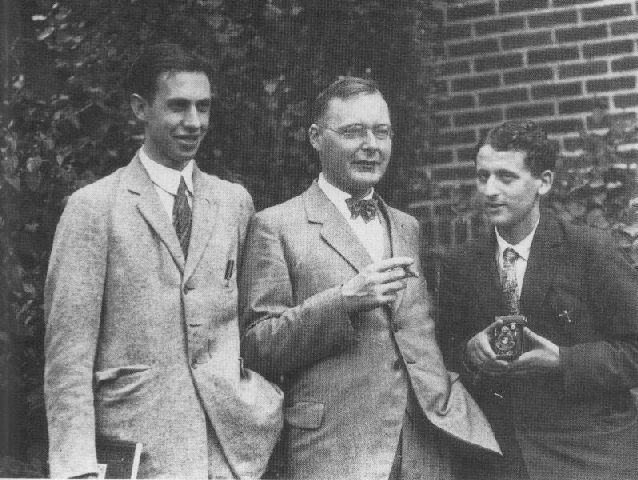
In 1925, two Dutch physicists, George Uhlenbeck and Samuel Goudsmith theoretically deduced the physical nature of "spin" from the experiment conducted by Otto Stern and Walther Gerlach to determine the magnetic moment of the electron present at the ‘s’ Orbital.
They chose silver as the electron source as it has $4S_{1}$ valence electronic configuration. The electron emitted is passed through a non-uniform magnetic field and then it’s allowed to strike the photographic plate on which the bands appear corresponding to the emitted electron’s magnetic quantum number i.e., ‘m’. The ‘S’ orbital has the value of the magnetic quantum number to be 0, so the electron’s path through the magnetic field should be straight without getting deviated since it has zero magnetic moment thus should result in a single band of light observed on the photographic plate. But here’s the catch. There were two bands that were observed on the photographic plate on deeper inspection. The angular momentum taking the values ‘-$\frac{\hbar}{2}$’, ‘0’ and ‘$+\frac{\hbar}{2}$’ (since electron possess half-integer spins $-\frac{1}{2}$ and $+\frac{1}{2}$)
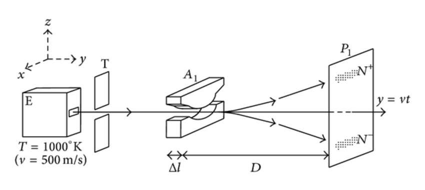
This result was attributed to being the unexplained parameter called “spin” by Pauli. From this experiment, Spin was defined to be an intrinsic form of angular momentum possessed by the elementary or quantum mechanical particles. Mathematically, he also devised a set of spin operators called Pauli Spin Matrices which act on the state vectors and gives an output. The spin matrices as follows,
$$\sigma_{x} = \begin{pmatrix}0 & 1 \\1 & 0 \end{pmatrix} \\~\\ \sigma_{y} = \begin{pmatrix}0 & -i \\i & 0 \end{pmatrix} \\~\\ \sigma_{z} = \begin{pmatrix}1 & 0 \\0 & -1 \end{pmatrix}$$
This experimental model was later used to find the spin values for various particles like protons, neutrons, neutrinos etc.
Entanglement
Tensor Product in Quantum Mechanics
In the context of our area of interest, which is quantum mechanical systems and quantum states, Tensor product is used to describe systems containing multiple subsystems wherein each subsystem is described by a vector in a vector space which in this case is a Hilbert Space. Say we have a state $|A \rangle$ and another state $|B\rangle$then the tensor product of these two states can be written as $|A\rangle \otimes |B\rangle = |AB\rangle$.
So, the |AB⟩ is an example of a combined state. When performing a tensor product between any two states, the states can be of any type of vector space. For example, Let’s consider a system of a coin, we have two possible states in this case that is, Heads and Tails and are represented as $|H\rangle$ , and $|T\rangle$. Next, we consider another system of a dice, we have 6 possible states ranging from 1 to 6 represented by $|1\rangle , |2\rangle$ and so on till $|6\rangle$. So, if we were to perform a tensor product between the states of these two systems, we would have the states of the resulting vector space to be $|H1\rangle, |H2\rangle$ and so on till $|H6\rangle$ and $|T1\rangle, |T2\rangle$and so on till $|T6\rangle$. The first half of the state label describes the state of the first system which in this case is the state of the coin and the second state label describes the state of the second system which in this case is the state of the dice.
Now, let's have a look at the properties of the said tensor product when applied to a quantum mechanical system. Let’s consider two systems ‘A’ and ‘B’ to be a penny and a dime. The person representing system A receives a penny or a dime at random and the same goes for the person representing system B. Let $\sigma$ represent the operator acting on the system to give an output. So, there’s a 50-50 chance of both the systems to receive a penny or a dime. Let’s consider that when $\sigma$ acts on $|Penny\rangle$ it gives the result “+1” and when it acts on $|Dime\rangle$ it gives the output “-1” and hence the expectation value of the operator $\sigma$ will be,
$\langle \sigma_{A} \rangle = 0 , \ \langle \sigma_{B} \rangle = 0$. But, $\langle \sigma_{A} : \sigma_{B} \rangle = -1$, since, at every point of observation, either system A or B will receive a dime hence the expectation value results in –1.
Hence, $\langle \sigma_{A} : \sigma_{B} \rangle = -1 \neq \langle \sigma_{A}\rangle :. \langle\sigma_{B} \rangle$ .
Two-Spin States
Let’s consider the spin pairs |u⟩ and |d⟩. Let the spin of system ‘A’ to be ‘$\sigma$’ and ‘$\tau$’ for system ‘B’. Let the basis for the combined system of these two spin states be $|uu\rangle, |ud\rangle, |du\rangle, |dd\rangle$⟩. From what we have discussed previously if $\sigma$ acts on $|u\rangle$, it gives us “+” and “-” for $|d\rangle$. The same is the case with $\tau$. Hence, we have the below set of equations
$$\sigma |uu\rangle = |uu\rangle\\\sigma |ud\rangle = |ud\rangle\\\sigma |du\rangle = -|du\rangle\\\sigma |dd\rangle = -|dd\rangle\\\tau |uu\rangle = |uu\rangle\\\tau |ud\rangle = -|ud\rangle\\\tau |du\rangle = |du\rangle\\\tau |dd\rangle = -|dd\rangle $$
As we can see in the above equations, the result of the $\sigma$ operator acting on the combined states only depends on the state that is present in the first half of the state label. The same is the case with the $\tau$ operator.
Quantum entanglement is a quantum mechanical phenomenon that occurs when a pair or group of particles interact, or share spatial proximity in a way such that the quantum state of each particle of the pair or group cannot be described independently of the state of the others. In other terms it is to say that the combined quantum mechanical System cannot be represented as a tensor product of the individual states of their respective systems. Now we shall see as to why that's the case with the combined states of a quantum mechanical system.
Entangled States
The states need not necessarily be a completely entangled state or not an entangled state at all. In entanglement, we can have various kinds of entangled states by themselves. We can have a maximally entangled state or a relatively strong entangled state or a weak entangled state. The strength of entanglement can vary depending on the nature of the particle.
The maximally entangled state is called as a singlet state. It is mathematically represented as,
$$|sing\rangle = \frac{1} {\sqrt{2}} (|ud\rangle - |du\rangle) $$
The singlet state cannot be written as a product state as it would just result in zero.
There are three more maximally entangled states called the triplet states. They can be represented as
$$\frac{1}{\sqrt{2}} \ (|ud\rangle + |du\rangle) \\ \frac{1}{\sqrt{2}} \ (|uu\rangle + |du\rangle) \\ \frac{1}{\sqrt{2}} \ (|uu\rangle - |dd\rangle)$$
There is a reason why the triplet states are mentioned separately from the singlet state. We shall look into that in a little while.
Let us recollect the example of the penny and the dime systems and how we found out that the expectation values of the operators resulted in zero. The same case applies to the spin pairs.
$$\langle \sigma_{x} \rangle + \langle \sigma_{y} \rangle + \langle \sigma_{z} \rangle = 0$$
The spin polarization principle is the degree to which the spin, i.e., the intrinsic angular momentum of elementary particles, is aligned with a given direction. In accordance with the spin polarization principle, there has to exist a spin component which aligns itself along a given reference direction and thus giving the output "+1". Hence, the sum of the expectation values of the individual spin pairs is,
$$\langle \sigma_{x} \rangle + \langle \sigma_{y} \rangle + \langle \sigma_{z} \rangle = 1$$
The above condition tells us that not all the expectation values can be zero.
This holds true for all product states. However, the singlet state, which is not a product state, doesn’t follow the rules of the Spin Polarization Principle. In fact, the RHS for the $|sing\rangle$ state results in zero.
We know that,
$$|sing\rangle = \frac{1} {\sqrt{2}} (|ud\rangle - |du\rangle) $$
To evaluate $\langle \sigma_{x} \rangle$, we take the singlet state as the basis.
$$\langle \sigma_{z} \rangle = \langle sing | \sigma_{z} | sing \rangle$$
So,
$$\langle \sigma_{z} \rangle = \langle sing | \sigma_{z} | sing \rangle = \langle sing | \frac{\sigma_{z}}{\sqrt{2}} | ud \rangle - |\frac{1}{\sqrt{2}} |du \rangle$$
or,
$$\langle \sigma_{z} \rangle = \langle sing | \sigma_{z} | sing \rangle = \langle sing | \frac{\sigma_{z}}{\sqrt{2}} | ud \rangle + |\frac{1}{\sqrt{2}} |du \rangle$$
Similarly,
$$\langle \sigma_{z} \rangle = \frac{1}{2} (\langle ud| - \langle du|) (|ud \rangle + |du \rangle)$$
$$\langle σ_{x} \rangle = \langle σ_{y} \rangle = \langle σ_{z} \rangle = 0$$
with the basis as the singlet state. If the expected value of a component of σ is zero, it means that the experimental outcome is equally likely to be “+1” or “-1”. In other words, the outcome is uncertain. Despite knowing the exact state vector, $|sing\rangle$, we know nothing about the outcome of any measurement of any component of either spin or it could also mean that we as observers do not completely know all the details that there is to know about |sing⟩. But according to the rules of quantum mechanics, there is nothing that can be known beyond the state vector that is encoded in $|sing\rangle$. The state vector gives us a complete description of the system that is possible to make. This thought bugged Einstein so much that he considered this phenomenon as “spooky action at a distance” as we can know everything there is to know about the system but can never know or understand the properties of its individual constituents.
The reason why the singlet is described separately is that the singlet is an eigenvector with one eigenvalue whereas, the triplets are all eigenvectors with different degenerate eigenvalues.
Quantum entanglement is a strange and spooky phenomenon that threw off our understanding of the quantum realm and also has shown us how strange quantum particles can behave.
The EPR paradox is a result of this phenomenon that states that each particle is individually in an uncertain state until it is measured, at which point the state of that particle becomes certain. The reason this is considered as a paradox is that the particles had to communicate the information to each other at speeds faster than the speed of light which again violates the law of Relativity.
Quantum Mechanics consists of more such phenomena that just don’t seem to make sense when we try to comprehend and try to make sense of it. Definitely, it is because it isn’t completely deterministic like classical physics and the minimum act of observation destroys the information that was once available in the system. We are bound to encounter more such strange phenomenon as we try to understand the nature of the quantum realm which makes us question our preconception of reality and also could show us how much it could differ from the actual truth.
Ackowledgements
The authors would like to thank Prof. Joseph Prabagar for inspiring us to write this article and Prof. Geno Kadwin for his insights into the mathematical aspects. A shoutout to Aishwarya Girish Kumar for her comments on the first draft.
References
- Shankar, R. (2014). Principles of quantum mechanics. New York, NY: Springer.
- Jeevanjee, N. (2016). Introduction to tensors and group theory for physicists. Birkhauser Verlag AG.
- Sakurai, J. J., & Napolitano, J. (2021). Modern Quantum Mechanics. Cambridge: Cambridge University Press.
- Kumar, M. (2008). Quantum: Einstein, bohr, and the great debate about the nature of reality. London: Icon Books.
- Susskind, L. and Friedman, A. Quantum Mechanics: The Theoretical Minimum. Basic Books, 2014