Charting The Stars

Modern astronomy has evolved a lot. It's no longer the field populated with cranky old men who fill their garages with lenses and telescopes. No. At the heart of the field that aims to chart out the cosmos lies something far more valuable than measurement apparatus –  data.

With the amount of information that we receive from various telescopes and from various sources, we cannot further rely solely on manpower in order to map the universe (in case you didn't know, it's a pretty big place).

So, as human have been doing for at least the last half-century, we offload tasks of detection, classification and interpretation to computers.

In this article, we're going to talk about some of the techniques that modern astronomers use day-to-day to handle the large influx of observational data, and how these computational techniques hold a lot of promise for further enhancing our perception of the universe in the future.

Image Stacking

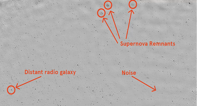
Often in astronomy we try to detect signals in the presence of noise. We usually work with grayscale images where black points are high flux density and gray area is the background noise. Most of the black dots you see in an image are distant radio galaxies. But some are objects in our own galaxy, such as pulsars or supernova remnants.

In radio astronomy, flux density is measured in units of Janskys (a unit which is equivalent to $10^{-26}$ watts per square meter per hertz).

In other words, flux density is a measure of the spectral power received by a telescope detector of unit projected area. In the grayscale image picked up by our telescope, we're interested in measuring the apparent brightness of a pulsar at a given frequency.

We typically call something a "detection" if the flux density is more than five standard deviations higher than the noise in the local region. So if we look for radio emission at the location of all known pulsars, sometimes we find detections, but most of the time we don't.

When we don't detect something, it could be for a lot of reasons. The pulsar could be too far away, the intrinsic emission may not be strong at these frequencies, or the emission could be intermittent and switched off at the time we measure it.

Now you might think we can't say anything about the pulsars we don't detect. After all, how can we derive anything from a non-detection?

However, astronomers have developed clever techniques for doing just that. One of which is stacking.

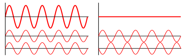
It allows us to measure the statistical properties of objects we can't detect. Stacking works because the noise in a radio image is roughly random, with a Gaussian distribution centered on zero. When you add regions of an image that just have noise, the random numbers cancel out. But when you add regions of an image in which there are signals, the signals add together, and thus increasing the signal to noise ratio.

The undetected pulsars are located all over the sky and so, to stack them we first need to shift their positions so they're centered on the same pixel. Our stacking process looks something like this. To calculate the mean stack, we just take the mean of every pixel in the image and form a new image from the result.

Bin Approx Algorithm

When we implemented median stacking, we ran into the problem of memory usage. Our naive solution involved keeping all the data in memory at the same time, which required much more memory than was available on a typical computer.

There are different solutions to this problem. Some of them require more money. Some require re-framing the problem. Some involve developing a smarter solution.

Perhaps, the simpler solution (although it does require the 💵) is to buy a better computer. To some extent this is a good solution, but of course as soon as the data size increases, we'd be back to the same problem.

The third approach is to improve our algorithm. Currently the problem is that calculating the median requires us to store all the data in memory. Can we calculate a running median that doesn't need all of the data to be loaded in memory at the same time?

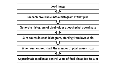
A solution to this is the bin approx. algorithm, which works as follows.

As each image comes in, take the value of each pixel in the image and place it in a bin. Once all of the images have been processed, you end up with a histogram of counts for each pixel in the image. Because the bins in the histogram are ordered, you can sum up the counts in the histogram starting from the smallest bin until you get to half the total number of numbers. You then use the value of the resulting bin as your median.

To put some real numbers in this example, let's generate 1,000 random numbers from a normal distribution. When we apply the bin approx. algorithm, we end up finding a mean of zero, which is what we'd exactly expect. So, what happens when we do this stacking? We end up with an image that shows a clear detection in the central few pixels.

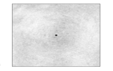
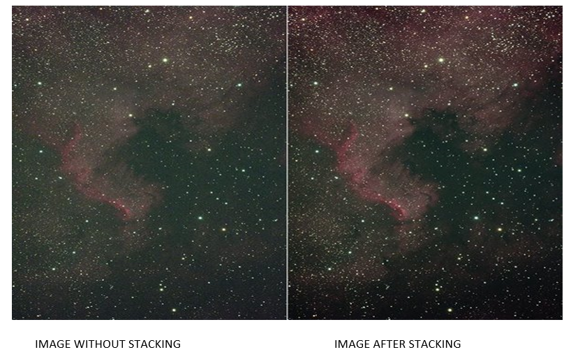
It may not look too impressive initially, but let's take a step back and think about what we're seeing here.

We took a large set of images for which we could not detect any individual pulsars. When we lined the images up so all of the undetected pulsars are located in the center of image, and then calculate the median across all of the images, we can see a detection. What you're seeing here is a statistical detection of a population of pulsars that are too faint to see in our original data set.

We've used a really simple technique to probe a bit of the invisible universe that you couldn't otherwise see using telescope alone!

Cross Matching

When we create a catalog from survey images, we start by extracting a list of sources, galaxies, and stars using source-finding software. There are many different packages we can use (`sExtractor` is a common one), but most of them work in a similar way.

Basically, they run through the pixels in an image and find peaks that are statistically significant. Then, they group the surrounding pixels and fit a function, usually based on the telescope response, which is called the 'beam' or the 'point spread function'. This results in a list of objects, each of which has a position, an angular size, and an intensity measurement. The uncertainties on these measured values depend on things like noise in the image, the calibration of the telescope, and how well we can characterize the telescope's response function.

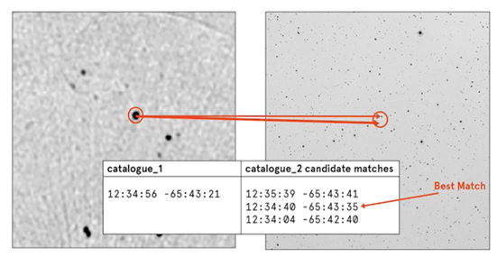
Once we have our catalogues, cross-matching involves searching the second catalogue to find a counterpart for each object in the first catalogue. To do this, we usually search within a given radius, based on the uncertainties in the position. For each source in the first catalogue, we look through each source in the second catalogue. We calculate the angular distance between each pair of sources, and if the angular distance is less than our search radius, and if that offset is the lowest we've seen so far.

When we run it on two catalogues, we end up with a list of matches between galaxies in the first catalogue, galaxies in the second catalogue and the great circles offset between them and we consider them a match.

Machine Learning in Astronomy

We know that humans are exceptionally good pattern matchers.

For example, research shows we can recognize other human faces within hundreds of milliseconds of seeing them. Perhaps it isn't surprising that we have these skills, our early survival depended on it. As scientists, we've adapted these skills to tasks such as the stellar spectral classifications. Often, human classifiers have a list of criteria or heuristics that they use to make decisions, combined with an overall intuition about the data.

So how can we train a computer program to do something we can't even express?

Early-on, researchers attempted to encapsulate this intuition with an unreasonnably large number of hard-coded rules to cover as many cases as possible. These types of systems can be successful, but they're slow to develop and they lack the ability to deal with unexpected inputs or ambiguous classes.

In contrast, machine learning algorithms don't depend on specific rules. Instead, they try to discover or learn patterns from input data we've given them. There are two broad types of machine learning algorithms, unsupervised and supervised.

Unsupervised algorithms try to discover patterns in data whereas supervised algorithms learn from classified input data, so they can classify unknown examples. For example, in the context of astronomy,  let’s consider the red shifts for the training data were calculated using spectroscopic techniques, which are generally a highly reliable way of calculating red shifts. In other cases, you might use a gold standard data set classified by human experts. Another option is to use training data classified by many non-experts. Galaxy Zoo is a massive citizen science project that has made scientific discovers through the work of dedicated amateurs and intelligent machine learning methods. So, the next step is to extract features that represent your input data in some way. We classify these features into the properties of various objects and use the decision trees to come up with a solution using these classifications. So, you've selected features that can be used to represent these objects using which you can train your classifier on this known data set. The process of training basically consists of building a model between your inputs and the result. This obviously will lack in accuracy for the first couple of thousands of data sets but as we keep feeding more and more inputs to the algorithm, the accuracy also increases along with it. The more we train the machine the more the machine can further classify the unknown object with great accuracy.

Decision Tree Classifiers

Decision trees are probably the easiest machine learning algorithm to understand, because their representation is similar to how we'd like to think a logical human might make decisions.

Let's consider an example: Should I play tennis today?

A machine "learns" how to make this decision based on training data from past experience.

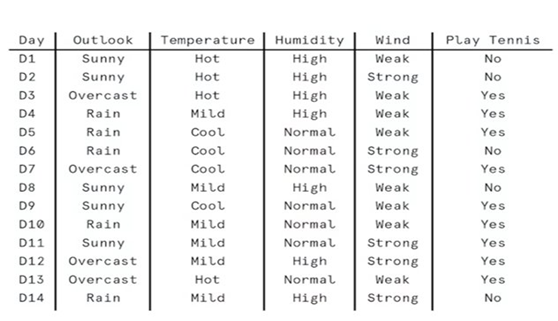
Let’s say the decision to play tennis depends entirely on four factors: the general weather outlook (sunny, overcast, or raining), the temperature (hot, mild, or cool)  humidity (high or low), and the wind (strong or weak).

For training data, we've tracked the decisions that we made on previous days of tennis playing. For example, day nine, a cool but sunny day with normal humidity and weak winds, was a good day for tennis. Day 14, with rain and strong winds, was not a tennis day.

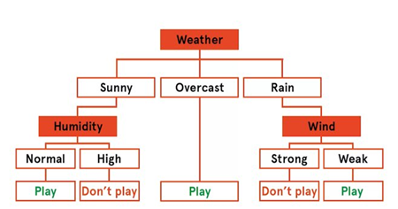
Based on this small data set, you could construct a decision tree by hand to work out when you should play tennis.

There are three options for the overall outlook, sunny, overcast, or rain. Based on this training data, we always play tennis when it's overcast. So that branch of the tree goes directly to a final leaf which assigns the classification play. If it's sunny, then our decision depends on the humidity. Sunny days with normal humidity are good for tennis. But sunny days with high humidity are not. Finally, if it's raining our decision depends on the wind. On rainy days with weak wind we can still play tennis, but rain plus strong winds are not enjoyable.

So that's how we could build this decision tree for this simple data set by hand. But how does the machine learning algorithm know which attributes to select at each level of the tree?

Informally, for each decision in the tree, the learner chooses a question that maximizes the new information or minimizes the error. Different algorithms use different metrics to measure this information gain.

Entropy measures how predictable or uncertain a distribution is. If the outlook is overcast, we always play tennis. So, we have complete certainty, and entropy equals zero. If the outlook is rain, we only predict we'll play tennis 60% of the time giving an entropy close to one. Information gain measures how much entropy is reduced by answering a particular question.

Once the algorithm has built the tree, you then apply this model to unknown data. In real world machine learning problems, you typically have thousands of training instances, making our predictions more robust.

Now, in this example, all of the features have been categorical data. The temperature could be hot, mild, or cool. Nothing else.

But in astronomy, most of our data will be real-valued.

Rather than having cool, mild, and hot, we now have temperatures ranging from 15 to 30 degrees Celsius, or about 60 to 90 degrees Fahrenheit. In this case, the learner follows roughly the same process, except that it needs to make decisions in the real value temperature space.

Instead of splitting by a particular value or category, a decision tree with continuous variables needs to learn "less than" and "greater than" rules such as "if the temerature is greater than 80, take the left branch."

Supervised learning can be used for either classification or regression. This tennis tree is an example of classification because the results are distinct categories, but we can also learn a decision tree with real valued results. One application of this method is using decision tree regression to calculate the red shift of galaxies.

Ensemble Classification

The decision tree approach is great, but in practice, we found it hard to get accurate results due to the presence of excessive noise from the data from the telescopes or from galaxy zoo.

So, in order to increase the reliability of the program we use a technique called ensemble learning where multiple models are trained and their results are combined together in some way.

The premise of ensemblig is that the combined classifications of multiple weak learners can give a more reliable and robust result than a single model's prediction in the face of imperfect training data.

For ensembles to work better than individual classifiers, the members of the ensemble must be different in some way. They must give independent results. If they all gave the same predictions on each instance, then having more of them would make no difference at all.

There are many ways to achieve this model independence, including using different machine learning algorithms, different parameters, for example the tree depth, or different training data.

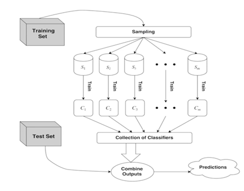
One of the most popular methods is called bootstrap aggregating, or bagging for short. In bagging, samples of the training data are selected with replacement from the original training set. The models are trained on each sample. Bagging makes each training set different with an emphasis on different training instances.

A random forest classifier is a supervised machine learning algorithm that uses an ensemble of decision tree classifiers. It builds an ensemble by randomly selecting, either subsets of training instances, bagging, or selecting a subset of features of each decision point.

The nice thing about a random forest is that we can use it pretty much everywhere we use a decision tree. Yes, it does usually involve setting more parameters and more computationally intensive, but it usually gives us better results.

Because each classifier in the ensemble returns a vote, we can not only find the most popular category but we can look at the distribution of votes over all the categories. This allow us to calculate an estimated probability that our classification is correct and identify which test instances are particularly hard for the system to classify. These probabilities can also let you identify out liners, objects that are not similar to any of the training classes, which can be a great way of identifying those rare objects that need further scientific investigation.

Conclusion

With the help of computers, the process of interpreting astronomical data has become significantly easier and more efficient. The real takeaway here is how useful it is for ideas from one field to bleed into another.

When Galileo first pointed those aligned lenses to the sky, he saw the stars. But today, thanks to statistics, machine learning, and advances in computation, we see more of what this universe has to offer.

Much, much more...

It’s not that there are things that science can’t explain. You look for the rules behind those things. Science is just a name for the steady, pain in the ass efforts that goes behind it.