Hyperbolic Functions and Non-Hyperbolic Claims

Trigonometry. The high-school mathematician's nightmare.
When we first learn about trigonometry in school, it’s introduced as being all about right-angled triangles—it is after all the ratios of two sides of a right triangle, isn’t it? Soon, we realize that it isn’t, in fact, limited to just triangles; we redefine all our notions of trigonometry with the help of a unit circle. Specifically, we learn that if we were to parametrize the unit circle, $x^2 + y^2 = 1$, the coordinates of a general point on it can be represented as $x=\cos t$ and $y=\sin t$, with $t$ being the parameter.

But why stop with a circle? Why can’t we extend these ideas of parametrization to another common conic—the hyperbola? Trust me, by the time you get to the end of this article, you’ll agree with my claim that the hyperbola, a curve that doesn’t seem to show up much in our daily life, is actually much more common than we think.
Before we jump into this, however, let’s first play around with our traditional trigonometric functions: sine and cosine.
Euler’s formula, $e^{it} = \cos t + i\sin t$, gives us a neat, perhaps unexpected, relationship between the trigonometric functions and the exponential function. If we rearrange the terms a little, we arrive at the following results:
$$\cos t = \frac{e^{it} + e^{-it}}{2}$$
$$\sin t = \frac{e^{it} - e^{-it}}{2i}$$
This seems a little odd; even if we just provide purely real values of $t$ as the input to the functions, the right-hand side seems to have something to do with imaginary numbers, although it does eventually simplify to give us real-valued outputs.
Also, as expected, these definitions of sine and cosine do indeed satisfy the equation $x^2 + y^2 = 1$. Don’t take my word for it. Pick up a pen and a piece of paper and square and add the functions and see for yourself.
So what if, just what if, we defined another pair of analogous functions based on these representations of sine and cosine, but this time, with all the imaginary units on the right-hand side removed?
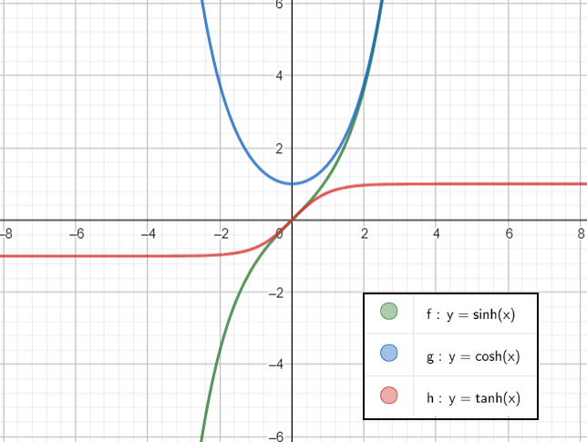
Let’s arbitrarily call these functions $\cosh$ (pronounced like kosh in kosher) and $\sinh$ (pronounced sinch or shine) respectively.
$$\cosh t = \frac{e^{t} + e^{-t}}{2}$$
$$\sinh t = \frac{e^{t} - e^{-t}}{2}$$
"Okay, but what does the $h$ stand for?" you ask? To find out, repeat the pen-and-paper process, but this time square and subtract the two instead. You should see, on simplifying, that $\cosh^2 t - \sinh^2 t = 1$.
It’s starting to make a little sense now, isn’t it?
If $x = \cosh t$ and $y = \sinh t$ are the parametric coordinates of a curve, the locus of all such points gives rise to the equation $x^2 - y^2 = 1$, which is simply the equation of a unit hyperbola! This is the very reason we call these functions the hyperbolic cosine and the hyperbolic sine.
We can then go on to define other hyperbolic functions like $\tanh$ and $\text{sech}$ just like we did for their circular counterparts. These functions satisfy identities analogous to those of the ordinary trigonometric functions (which I would encourage you to derive).
Circular Analogies
Looking back at the traditional circular trigonometric functions, they take as input the angle subtended by the arc at the center of the circle. Similarly, the hyperbolic functions take a real value called the hyperbolic angle as the argument. To understand hyperbolic angles, we first need to think about traditional angles in a slightly different way.
If an arc of a unit circle subtends an angle of $\theta$ radians, then the area of the corresponding sector is $\frac{\theta}{2\pi} \times \pi$ or $\frac{\theta}{2}$. In other words, the angle is equal to twice the area of the sector.
Analogous to this, a hyperbolic angle is twice the area of the corresponding hyperbolic sector (which, like its circular counterpart, is simply the region enclosed by rays from the origin to two points on the hyperbola). This means that if you choose a point ($\cosh t$, $\sinh t$) on the unit hyperbola, the line segment joining the point with the origin creates a sector of area $\frac{t}{2}$ with the x-axis and the hyperbola.
The main point to keep in mind here is to visualize hyperbolic angles with the help of areas, not as a figure created by two rays as you might imagine normal angles. From this, it also arises that hyperbolic angles are unbounded, as the area of the sector keeps increasing as the point moves farther and farther away from the origin, which is not the case for circular angles.
Why Should I Care?
Take a piece of rope and suspend it from two rigid stands. What geometric shape do you observe the rope taking up?
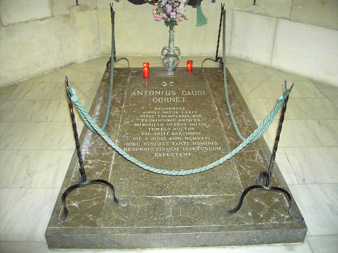
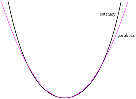
If you said parabola, I don’t blame you; I thought so too at first. And so did Galileo! But as it turns out, this shape is actually a catenary, the shape of the hyperbolic cosine function. It happens to appear to be strikingly similar to a parabola, but it isn’t quite the same.
To prove this, let’s consider a point $P(x,y)$ on the rope, separated from the bottom-most point $O$ on the rope by an arc of length $l$. Let $\lambda$ be the rope’s linear mass density.
If we consider the section of the rope between $O$ and $P$, it is in equilibrium due to three forces: the two tensions ($T_0$ and $T_P$) pulling it outwards at either end and gravity pulling it downwards.
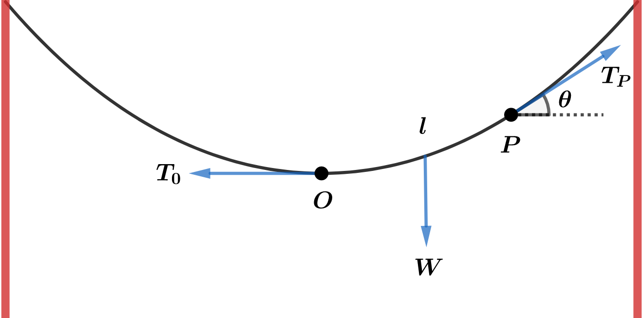
As the section is in equilibrium, the net forces in the horizontal and vertical directions must each be zero. Hence we obtain the following relations:
$$W = \lambda lg = T_P \sin \theta$$
$$T_0 = T_P \cos \theta$$
This in turn gives:
$$\tan \theta = \dfrac{\lambda lg}{T_0}$$
In the right hand side of the above equation, the terms $\lambda$, $g$ and $T_0$ are all constants, so we can replace them with a single constant $a = \frac{\lambda g}{T_0}$. Also, $\tan \theta$ is nothing but the slope of the curve, $\frac{dy}{dx}$. Hence:
$$\dfrac{dy}{dx} = al$$
Differentiating this, we get:
$$\dfrac{d^2y}{dx^2} = a \dfrac{dl}{dx}$$
The small arc length $dl$ can be considered to be approximately a straight line segment, and hence the hypotenuse of a right triangle, with the other two sides being $dx$ and $dy$. Using the Pythagoras Theorem on this triangle yields the following relation:
$$dl^2 = dx^2 + dy^2$$
Dividing both sides by $dx^2$ and then taking the square root on both sides gives the following expression for $\frac{dl}{dx}$ which we can then substitute in the previous equation:
$${\left(\dfrac{dl}{dx}\right)}^2 = 1 + \left(\dfrac{dy}{dx}\right)^2$$
$$\dfrac{dl}{dx} = \sqrt{1 + \left(\dfrac{dy}{dx}\right)^2}$$
$$\dfrac{d^2y}{dx^2} = a \sqrt{1 + \left(\dfrac{dy}{dx} \right)^2}$$
This is nothing but a second order differential equation, which we can solve by making the substitution $z = \frac{dy}{dx}$, and then using the variable separable method.
$$\dfrac{dz}{dx}= a \sqrt{1+z^2}$$
$$\int \dfrac{dz}{\sqrt{1+z^2}} = \int {a} {dx}$$
$$\ln (z + \sqrt{1+z^2}) = ax + c$$
When $x = 0$, $z = \frac{dy}{dx} = \tan 0 = 0$, and we can hence safely set $c$ to 0. From here, it's just a matter of simplifying the equation and finding the value of $z$ as:
$$z = \dfrac{dy}{dx} = \dfrac{e^{ax}-e^{-ax}}{2}$$
The right hand side of this equation is starting to look a little familiar, isn't it? We're getting close to the answer! The last step is to once again solve the above differential equation (the constant of integration can be ignored as we are free to move the coordinate axes and set them to a position at which $c = 0$).
$$\int dy = \int \dfrac{e^{ax}-e^{-ax}}{2} dx$$
$$y = \dfrac{e^{ax}+e^{-ax}}{2a} = \dfrac{\cosh {ax}}{a}$$
And there you have it! We have just successfully shown that the rope does take the shape of a catenary and not a parabola, with the constant $a=\frac{\lambda g}{T_0}$ determining the exact shape.
So hyperbolas and hyperbolic functions do indeed manifest in various (albeit somewhat hidden) ways in everyday life. Of course, dangling ropes and barricade poles are just some examples of where you might encounter these functions.
They also happen to be used in machine learning and neural network applications, as well as in non-Euclidean geometry, for example in maps that use the Mercator projection (look up the sigmoid function and the Gudermannian function to find out more). My initial claim that hyperbolas are much more common than we think is therefore clearly no hyperbole.
Q.E.D.